Agriculture Financial Model in Excel (Free Farm & Crop Download)
An agriculture financial model projects crop revenue (acres × yield × price) and livestock income against input costs near 55% of revenue, machinery CAPEX and seasonal working capital, producing linked statements with valuation. Generate a 16-sheet Excel farm model free for up to 3 years.
⚡ Generate my Agriculture model — free (requires JavaScript)
The fastest way to an investor-ready agriculture financial model is a template pre-loaded with the industry's real revenue drivers and cost structure. This generator builds a 16-sheet, fully formula-linked Excel workbook — three statements, DCF & IRR — around agriculture-specific assumptions in about five minutes. Free up to 3 years, just your email.
Key drivers pre-loaded in this template
| Acres × yield × price | Crop revenue build |
| Livestock & dairy stream | Diversified farm income |
| Machinery CAPEX $1.2M default | Equipment with depreciation schedules |
| Input costs ~55% | Seed, fertilizer, feed and labour |
What you get
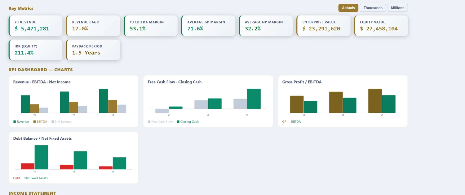
A 16-sheet, fully formula-linked Excel workbook: Assumptions, Revenue, OPEX, CAPEX & Depreciation, Debt, Tax (with loss carryforward), Income Statement, Cash Flow, Balance Sheet, DCF Valuation, Sensitivity tables, a charted KPI Dashboard, a Scenarios sheet (Base, Best & Worst), and an Integrity Check. Free 16-sheet linked Excel download for models up to 3 years (annual or quarterly, just your email). Models from 5 to 25 years are $29.98 per model download.
What an agriculture financial model computes
Farming is a business of biological timing and price volatility, and the model exists to make both legible. Revenue is acres multiplied by yield multiplied by price for crops, or head multiplied by weight and price for livestock, and two of those inputs move with forces no farmer controls. Against revenue sit the inputs bought at planting, the machinery that does the work, and the land underneath it. The two forces that decide the outcome are yield and price on the revenue side, and the seasonal cash cycle on the finance side, because spending leads revenue by months. A generic template flattens the volatility and ignores the seasonality, missing exactly what makes farm finance hard.
The template loads farm-scale defaults: crop or livestock revenue driven by yield and price, input costs through the season, machinery on the CAPEX schedule, and a working-capital cycle that peaks before harvest. What follows is what each part does with real agricultural numbers in it.
Farm types change the model
Before any numbers, the enterprise type sets the revenue rhythm and the cost base.
| Type | Revenue basis | Cash rhythm | Modelling focus |
|---|---|---|---|
| Row crops | Acres × yield × price | One or two harvests a year | Yield, price, input timing |
| Livestock | Head × weight × price | Steadier, feed-driven | Feed cost, weight gain, cycle |
| Permanent / orchard | Trees × yield × price | Years to first crop | Establishment CAPEX, ramp |
| Mixed / rotation | Blended streams | Smoothed across crops | Rotation, diversification |
Row crops are the classic seasonal case: cash goes out at planting and comes back at harvest, so the funding trough is deep and predictable. Livestock smooths the rhythm, with feed as the dominant variable cost and weight gain the revenue driver, but ties up cash in the animals. Permanent crops like orchards and vineyards invert the timing entirely, demanding heavy establishment capital and several years before the first commercial crop, so the model has to carry a long ramp. The template keeps the enterprise explicit because the cash shape is completely different across them.
Revenue: the three numbers that multiply
Crop revenue is deceptively simple and genuinely volatile, because two of its three drivers are set by nature and markets.
| Driver | Set by | Volatility | Modelling note |
|---|---|---|---|
| Acres | The farmer | Controlled | The one input you decide |
| Yield per acre | Weather, inputs, soil | High | Stress across seasons |
| Price per unit | Global markets | High | Often hedged forward |
Acres are the only lever fully in the farmer's hands. Yield swings with weather and agronomy, and price swings with global supply and demand, and the two are only loosely linked, which is why a great growing season can meet a weak market. Forward contracts and hedging can lock some price in, and the model keeps price and yield separate so the effect of a hedge, or its absence, is visible rather than buried. This is the same volatility that makes a multi-year view essential.
The four assumptions that decide farm returns
| Assumption | Typical range | Why it dominates |
|---|---|---|
| Yield per acre | Crop-dependent | Multiplies straight into revenue |
| Commodity price | Market-dependent | The most volatile driver |
| Input cost per acre | Seed, fertiliser, fuel | The controllable margin lever |
| Machinery CAPEX & life | Long-lived equipment | Depreciation and replacement cash |
Yield and price multiply directly into revenue and are the two the farmer controls least, so the model treats them as the primary stress variables. Input cost per acre is the margin lever the farmer does control, and in a low-price year it is often the difference between a small profit and a loss. Machinery CAPEX and its long life set the depreciation and the replacement cash a multi-year plan has to fund. Get honest ranges on these four and the model does the rest.
Worked example: a 2,000-acre row-crop farm, in numbers
| Input | Value |
|---|---|
| Acres | 2,000 |
| Yield per acre | 180 bu |
| Price per bushel | $5.00 |
| Crop revenue | $1.8M |
| Input cost per acre | $450 |
| Total input cost | $0.9M |
| Machinery CAPEX | $1.2M, 10-yr life |
| Operating margin | after inputs & overhead |
| Cash trough | before harvest |
From yield to margin and IRR
2,000 acres at 180 bushels an acre is 360,000 bushels, and at $5 that is $1.8M of crop revenue. Input costs at $450 an acre take $0.9M, so the gross over inputs is about $0.9M, from which machinery depreciation, land cost and overhead are taken to reach operating profit. The sensitivity is stark: drop yield to 150 bushels or price to $4.20 and the margin can halve or vanish, which is why the model stresses both and why one good year proves nothing. Cash tells its own story, bottoming out just before harvest when a full season of inputs has been spent and nothing has yet sold, and that trough is the operating line the farm must have in place before planting. Over a 3 to 25-year horizon the model funds the machinery replacement, carries the seasonal swing, and produces the DCF and IRR across a run of seasons rather than a single lucky one.
Land: the asset beneath the business
No other business rests on an asset quite like farmland, and the model has to decide how it is held. An owner-operator carries the land on the balance sheet, where it depreciates little or not at all and often appreciates, so a farm can build real equity even in lean operating years as land value compounds underneath a thin operating margin. A tenant farmer pays rent instead, turning a large fixed asset into an annual cost that eats directly into margin but frees up capital. The choice reshapes the whole model: owned land means a big balance sheet, mortgage debt and land equity that can dominate the return; rented land means a leaner balance sheet and a rent line that has to be covered every season regardless of yield or price. The template keeps land explicit, owned or rented, so the operating economics and the asset story are both visible, because for many farms the land is worth more than a decade of profit and quietly drives the total return.
Agriculture model vs a generic financial model
| What differs | Generic model | Agriculture financial model |
|---|---|---|
| Revenue driver | Price × volume | Acres × yield × price, both volatile |
| Volatility | Smooth growth | Yield and price stressed across seasons |
| Cash timing | Even | Seasonal, deep pre-harvest trough |
| CAPEX | Steady spend | Machinery on a replacement cycle |
| Horizon view | Single year | A cycle of good and bad seasons |
Sector-level income, yield and cost benchmarks for calibrating assumptions are published by the USDA Economic Research Service, the standard US series for farm income and finances.
Reference: USDA ERS — Farm Sector Income & Finances. For the seasonal cash view, use the agriculture cash flow model.
How to download your agriculture model (3 steps)
- Choose the Agriculture template. The acres, yield, price, input-cost and machinery defaults load as editable inputs.
- Set your own yields, prices, input costs per acre, machinery CAPEX and rotation. Pick annual or quarterly periods and a 3 to 25-year horizon.
- Preview the linked statements, margin, IRR and DCF, then download the Excel workbook. Up to 3 years is free with just your email; longer horizons are a one-time purchase.
Three focused variants build on the same agriculture engine: the agriculture cash flow forecasting model for the seasonal cash cycle, the agriculture DCF valuation model for enterprise value and IRR, and the agriculture free cash flow model for peak funding need.
Frequently asked questions
Can I model seasonality?
Use the quarterly mode to capture planting-to-harvest cash-flow timing across the year.
How are commodity price swings handled?
Set price inflation per growth band, and use the sensitivity sheet to test revenue × margin scenarios.
What horizon suits farm investment?
Annual operations plan over 3–5 years free; orchards, irrigation and land development appraise over 10–25 years with premium.
What drives revenue in a farm financial model?
Three numbers multiplied together: acres farmed, yield per acre, and price per unit. A 2,000-acre operation at 180 bushels an acre and $5 a bushel books $1.8M of crop revenue, and because two of those three inputs are outside the farmer's control, revenue is inherently volatile. The model keeps acres, yield and price separate so weather and market swings can be stressed independently rather than hidden in one growth rate.
How volatile is farm income, and how do you model it?
Very. Yield swings with weather and price swings with global markets, and the two are only loosely related, so a bumper crop can coincide with a price collapse. A single-year forecast tells you almost nothing. The model runs multiple years with yield and price as explicit, stressable drivers, so a rotation plan or a run of average seasons is judged across a cycle rather than on one good or bad year.
Why does a profitable farm need so much financing?
Timing. Inputs are bought and paid for at planting while revenue arrives months later at harvest, so cash bottoms out just before the crop sells. That seasonal trough is the operating line a farm must have committed before planting, and machinery adds term debt on top. A farm can be profitable every year and still need a large, well-structured facility to bridge the gap, which the model sizes explicitly.
Agriculture across our four models
Agriculture Cashflow Forecasting Model · Agriculture DCF Valuation Model · Agriculture Free Cashflow Model
More industry financial models
SaaS / Subscription financial model · Data Center financial model · Real Estate financial model · Manufacturing financial model · Hotel / Hospitality financial model · E-commerce / Retail financial model · Healthcare / Clinic financial model · Fintech / Lending financial model · Energy / Solar financial model · Early-Stage Startup financial model · Restaurant / F&B financial model · Professional Services financial model · Logistics / Transport financial model · Education / Training financial model · Construction financial model · Media / Content financial model · Telecom / ISP financial model · Pharma / Distribution financial model · Fitness / Wellness financial model · Nonprofit / NGO financial model · Pricing
Free tools
WACC calculator · CAPM calculator · DCF calculator · IRR calculator · Inside the 16-sheet model · Glossary