Solar Financial Model in Excel (Free PPA, LCOE & IRR Download)
A solar or energy financial model projects generation revenue (MWh × PPA rate) plus renewable-energy credits against panel and plant CAPEX, project debt and O&M costs. Because PPAs typically run 20–25 years, the premium tier models the full contract life; 3-year models are free.
⚡ Generate my Energy / Solar model — free (requires JavaScript)
The fastest way to an investor-ready energy / solar financial model is a template pre-loaded with the industry's real revenue drivers and cost structure. This generator builds a 16-sheet, fully formula-linked Excel workbook — three statements, DCF & IRR — around energy / solar-specific assumptions in about five minutes. Free up to 3 years, just your email.
Key drivers pre-loaded in this template
| MWh × PPA rate | Contracted generation revenue |
| REC income stream | Renewable-energy certificate sales |
| $3M CAPEX, project debt | Infrastructure financing structure |
| WACC ~10% | Contracted-cash-flow discount rate |
What you get
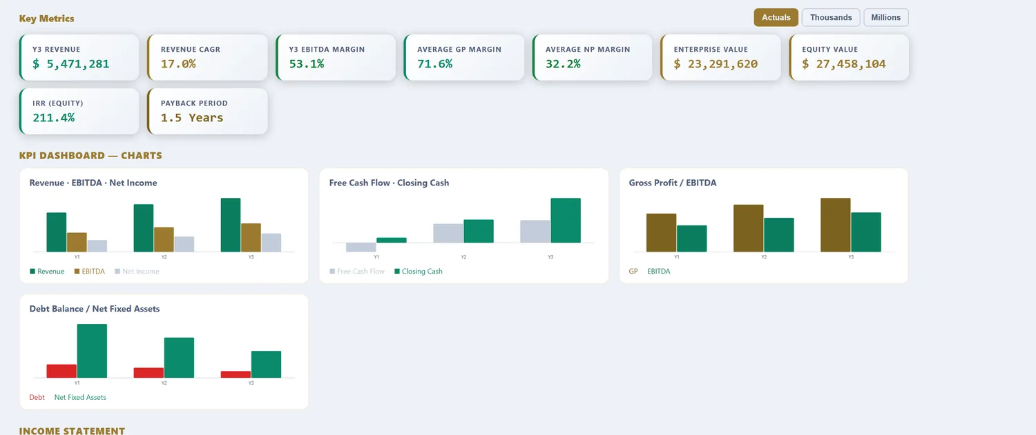
A 16-sheet, fully formula-linked Excel workbook: Assumptions, Revenue, OPEX, CAPEX & Depreciation, Debt, Tax (with loss carryforward), Income Statement, Cash Flow, Balance Sheet, DCF Valuation, Sensitivity tables, a charted KPI Dashboard, a Scenarios sheet (Base, Best & Worst), and an Integrity Check. Free 16-sheet linked Excel download for models up to 3 years (annual or quarterly, just your email). Models from 5 to 25 years are $29.98 per model download.
What a solar financial model actually computes
A solar project is a long-life asset with almost all its cost at the start and a thin, predictable revenue stream for 25 years after. That shape is what the model has to capture. Revenue is installed capacity in kilowatts-peak multiplied by the specific yield (how many kilowatt-hours each kWp produces in a year for the site's irradiance) multiplied by the tariff the electricity sells at. Against that sit the upfront CAPEX, the project debt that funds most of it, ongoing operations and maintenance, and panel degradation that quietly erodes output every year. Out of those inputs the model produces three numbers that decide whether the project gets built: the levelised cost of energy, the project internal rate of return, and a discounted cash flow valuation over the full asset life.
The template loads utility-scale defaults so the mechanics are visible from the first click: generation revenue driven by MWh and a PPA rate, a renewable-energy-credit income line, heavy CAPEX funded by project debt, and a horizon long enough to cover the whole contract. What follows is what each part does with real solar numbers in it.
The three system types, and how each one changes the model
Before any numbers, the system type sets the revenue logic. A model built for a grid-tied utility farm does not describe an off-grid installation, and forcing one shape onto the other is the most common way these forecasts go wrong.
| System type | How it earns | Storage | Modelling focus |
|---|---|---|---|
| Grid-tied | Sells all output to the grid or an offtaker | None or minimal | Yield, tariff, degradation, availability |
| Off-grid | Displaces diesel or grid power on site | Battery is essential | Load match, battery cycles and replacement |
| Hybrid | Self-consumes, exports the surplus | Battery, often with a genset | Self-consumption rate, export price, storage economics |
For a grid-tied plant the whole model is generation times price, so specific yield and the tariff carry it. An off-grid system earns by avoiding a cost rather than booking a sale, which means the battery is not optional: its cycle life and mid-life replacement CAPEX often decide the return. A hybrid sits between the two, where the split between self-consumed and exported energy sets the effective price, because power used on site is worth the retail rate you avoid while exports clear at a lower wholesale or feed-in price.
The hardware that drives the numbers
Solar economics are set by a small number of components, and each one moves a specific line in the model. You do not need to model every bracket, but the choices below change CAPEX per watt, annual yield, or the replacement schedule.
Panels: monocrystalline, polycrystalline, thin-film
| Technology | Efficiency | Cost | Model effect |
|---|---|---|---|
| Monocrystalline | 20-23% | Higher $/W | More kWp in the same area; higher yield, higher CAPEX |
| Polycrystalline | 15-18% | Lower $/W | More area for the same capacity; cheaper, lower density |
| Thin-film | 10-13% | Lowest $/W | Large land footprint; better in heat and diffuse light |
Efficiency decides how many watts fit in a given roof or field, so it sets both the installable capacity and the land or roof cost per watt. Monocrystalline dominates new build because higher efficiency lowers the balance-of-system cost that scales with area. In the model this shows up as the CAPEX per watt and the specific yield moving together.
Inverters: string, micro, central
The inverter converts DC panel output to AC and is the component most likely to need replacing inside the asset life. String inverters are standard for commercial and utility arrays and last around 10-15 years, which means at least one mid-life replacement the model has to fund. Microinverters sit on each panel, cost more up front, and suit shaded residential roofs. Central inverters serve the largest farms. Whatever the choice, the replacement CAPEX in year 10-15 is a real cash outflow that flatters the return if you leave it out, so the CAPEX schedule carries it explicitly.
Trackers and balance of system
A single-axis tracker follows the sun through the day and lifts annual yield by roughly 15-25% over a fixed mount, at higher CAPEX and more maintenance. Whether that trade earns its keep is a direct model question: the extra generation revenue against the extra cost and O&M. Balance of system, the mounting, wiring, combiner boxes, transformers and grid connection, is the unglamorous half of the budget and often approaches the module cost itself, which is why CAPEX per watt, not panel price, is the number that actually sizes the project.
Residential, commercial, and utility-scale
The same physics runs at three very different scales, and the model horizon and cost base shift with each.
| Segment | System size | Installed cost | Revenue basis |
|---|---|---|---|
| Residential | 3-15 kW | $2.50-3.50/W | Net metering or self-consumption |
| Commercial (C&I) | 100 kW-5 MW | $1.00-1.80/W | On-site PPA or net metering |
| Utility-scale | 5 MW-500 MW+ | $0.80-1.20/W | Wholesale PPA or merchant |
Cost per watt falls sharply with scale because fixed engineering, permitting and grid-connection costs spread across more capacity. A homeowner pays two to three times the per-watt cost a utility developer does, which is why residential economics lean on avoided retail power prices rather than wholesale sales. The commercial-and-industrial segment is where behind-the-meter PPAs live: a business hosts the array and buys the output below its grid tariff, and the developer earns the spread.
Revenue: PPA, feed-in tariff, or net metering
How the electricity is sold matters as much as how much is generated, because it sets both the price and the risk.
| Mechanism | Who pays | Price certainty | Financing effect |
|---|---|---|---|
| Power purchase agreement | A contracted offtaker | Fixed for 15-25 years | Bankable; supports high debt |
| Feed-in tariff | A utility or government scheme | Fixed by policy | Bankable while the scheme lasts |
| Net metering | The host, via avoided cost | Tracks the retail tariff | Depends on self-consumption |
A power purchase agreement is the foundation of project finance solar: a creditworthy buyer commits to a price for two decades, which lets lenders advance most of the CAPEX at a low rate. Feed-in tariffs did the same job through policy and built much of the early market. Net metering underpins residential and smaller commercial, where the value is the grid power you no longer buy. The model treats the PPA rate and the REC income as separate lines so a contracted price and a merchant tail can be blended when the offtake is shorter than the panel life.
The four assumptions that decide solar IRR
A solar model has many inputs but only a handful move the answer. Get these four honest and the rest is arithmetic.
| Assumption | Typical range | Why it dominates |
|---|---|---|
| Specific yield / capacity factor | 16-28% CF | Sets annual MWh from installed capacity |
| CAPEX per watt | $0.80-1.80/W (utility/C&I) | The whole investment base and debt size |
| Degradation | 0.4-0.7% per year | Compounds output loss across 25 years |
| Tariff + O&M escalation | PPA rate, 1-2% O&M growth | Net margin every single year |
Capacity factor is the conversion from nameplate megawatts to real megawatt-hours, and a two-point error runs straight through 25 years of revenue. CAPEX per watt sets the size of the investment and therefore the debt. Degradation looks small at half a percent but compounds: a panel producing 100% in year one is near 88-90% by year 25, and a model that holds year-one output flat overstates lifetime generation by roughly a tenth. Escalation on the tariff and on O&M decides whether the margin widens or narrows as the plant ages.
Worked example: a 5 MW commercial solar project, in numbers
| Input | Value |
|---|---|
| Installed capacity | 5,000 kWp |
| CAPEX at $1.10/W | $5.5M |
| Project debt (70%) | $3.85M at 7% |
| Equity | $1.65M |
| Specific yield | 1,600 kWh/kWp/yr |
| Year-1 generation | 8,000 MWh |
| PPA rate | $70/MWh, 1.5% escalation |
| O&M | $12/kW/yr |
| Degradation | 0.5% per year |
From megawatt-hours to project IRR
The plant generates about 8,000 MWh in year one, which at $70 per MWh is roughly $560,000 of revenue, plus a REC line on top. O&M runs near $60,000. After debt service on the $3.85M facility, the equity holder sees a rising cash yield as the loan amortises and the PPA escalator lifts the price faster than degradation cuts the volume. Over the 25-year life that profile produces an equity IRR in the low teens for a contracted utility or commercial project, which is the band infrastructure investors underwrite to. Push the capacity factor down two points or leave degradation out and that same project tells a materially different story, which is exactly why the sensitivity tables matter here more than in almost any other model.
Where LCOE comes from
Levelised cost of energy is the honest unit cost: lifetime discounted cost divided by lifetime discounted generation. For this project that lands in the region of $50-60 per MWh, comfortably under the PPA rate, and the gap is the margin. Utility-scale solar reaching the $30-60 range is what turned it into the cheapest new generation across much of the world, a shift documented year on year in the Lazard Levelized Cost of Energy analysis.
Benchmarks: Lazard LCOE+ for technology cost trends, and NREL cost benchmarks for US installed-cost data by segment.
Why degradation belongs in every year
A solar panel does not produce the same energy at 25 as it did at one. Manufacturers warrant a degradation rate, commonly around half a percent a year, and it compounds: year two is 99.5% of year one, year three is 99.5% of that, and by year 25 the array is delivering close to 88% of its first-year output. On a single year the effect is invisible. Across the asset life it removes roughly a tenth of total generation, and because it lands in the later years it hits the cash flows the terminal value depends on. The model applies it band by band across the 25-year horizon, so the late-life revenue is honest rather than a flat extrapolation of year one.
Solar model vs a generic financial model
| What differs | Generic model | Solar financial model |
|---|---|---|
| Revenue driver | Price × volume | kWp × specific yield × tariff, net of degradation |
| CAPEX shape | Steady annual spend | Almost all upfront, plus a mid-life inverter replacement |
| Output over time | Flat or growing | Declining every year at the degradation rate |
| Debt | Simple term loan | Project finance sized on contracted PPA cash flows |
| Horizon | 3-5 years | 20-25 years, the full contract and panel life |
How to download your solar model (3 steps)
- Choose the Energy / Solar template. The generation, REC, CAPEX and project-debt defaults load as editable inputs.
- Set your own capacity, specific yield, PPA rate, CAPEX per watt, degradation and O&M. Pick annual or quarterly periods and a horizon out to 25 years.
- Preview the linked statements, LCOE, IRR and DCF, then download the Excel workbook. Up to 3 years is free with just your email; the full 25-year life is a one-time purchase.
Three focused variants build on the same solar engine: the solar cash flow forecasting model for period-by-period liquidity, the solar DCF valuation model for enterprise value and IRR, and the solar free cash flow model for the CAPEX-to-FCF bridge and peak funding need.
Frequently asked questions
Why model a solar project over 25 years?
Solar assets earn contracted revenue across a 20–25 year PPA and panel life; IRR and DCF are only meaningful over the full horizon — exactly what the 25-year premium tier provides.
Does it compute project IRR?
Yes — equity IRR on post-debt cash flows, plus DCF enterprise value with Gordon-Growth terminal value.
Can I include degradation?
Approximate panel degradation by setting slightly negative or low volume growth in later growth bands.
How do you calculate solar LCOE?
Levelised cost of energy divides the project's lifetime discounted cost by its lifetime discounted generation. Add CAPEX, the present value of O&M and any debt cost, discount it, then divide by discounted MWh across the 25-year life, net of degradation. Utility-scale solar now lands near $30-60 per MWh, below most fossil generation.
What is a typical capacity factor for solar PV?
Fixed-tilt utility solar runs a 16-20% capacity factor in good irradiance regions; single-axis trackers push that to 24-28%. Residential rooftops sit lower, often 12-18%, because of orientation and shading. The figure sets how many MWh each installed megawatt actually produces in a year, which is the first number a lender checks.
Is a contracted PPA or a merchant model easier to finance?
A long-dated PPA with a creditworthy offtaker is far easier to finance: the revenue is contracted, so lenders advance more debt at a lower rate. Merchant projects sell into the spot market, carry price risk, and raise a higher equity share at a higher return. The model runs both so you can price the difference.
Energy across our four models
Energy / Solar Cashflow Forecasting Model · Energy / Solar DCF Valuation Model · Energy / Solar Free Cashflow Model
More industry financial models
SaaS / Subscription financial model · Data Center financial model · Real Estate financial model · Manufacturing financial model · Hotel / Hospitality financial model · E-commerce / Retail financial model · Healthcare / Clinic financial model · Fintech / Lending financial model · Early-Stage Startup financial model · Restaurant / F&B financial model · Professional Services financial model · Logistics / Transport financial model · Education / Training financial model · Construction financial model · Media / Content financial model · Telecom / ISP financial model · Agriculture financial model · Pharma / Distribution financial model · Fitness / Wellness financial model · Nonprofit / NGO financial model · Pricing
Free tools
WACC calculator · CAPM calculator · DCF calculator · IRR calculator · Inside the 16-sheet model · Glossary